Analyzing wait times for Halo Infinite - Anvil

July 31, 2024 in Data by Den Delimarsky6 minutes

The latest dataset for Anvil is now available on GitHub.

A bit less than a month ago I mentioned that I was aggregating wait time data for Halo Infinite events in open-source data sets. Yesterday, with the launch of the Fleetcom operation I’ve wrapped up the snapshotting of wait times for Anvil.

Get Anvil wait time data

Download the SQLite database.

Exploring the data

To get an idea of what the wait times were in the past operation, we can download the anvil-wait-times.db SQLite database. The data captures wait times in ten-minute increments since the day the operation started.

What data is captured?

Keep in mind that the data captured in the data set is representing wait times for the US West Coast. In future datasets I will explore the ability to capture data across other regions.

Once you download the database, you can use a tool like DB Browser for SQLite to peek inside the binary blob and see the structure and the contents.

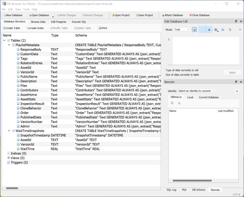
The structure of the database containing wait times for Anvil.

There are two key tables - WaitTimeSnapshots, that contains exact snapshots of wait times (in seconds) in ten-minute increments, and PlaylistMetadata, containing playlist details for each of the playlists active at the time of capture.

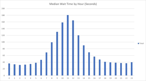
You can also run SQL queries on the data. For example, if you wanted to see the median (not average) wait times for BTB Sentry Defense by the hour over the entire span of the operation, you can filter by the appropriate asset and version IDs:

WITH HourlyWaitTimes AS (
    SELECT
        strftime('%H', datetime(SnapshotTimestamp)) AS Hour,
        WaitTime
    FROM
        WaitTimeSnapshots
    WHERE
        AssetId = '7961FD0C-0833-4565-8AF8-8E4B6F984EF5' AND
        VersionId = '15A55DBC-D0FE-419B-AB03-DADEC354616D'
),
RankedWaitTimes AS (
    SELECT
        Hour,
        WaitTime,
        ROW_NUMBER() OVER (PARTITION BY Hour ORDER BY WaitTime) AS RowNum,
        COUNT(*) OVER (PARTITION BY Hour) AS TotalCount
    FROM
        HourlyWaitTimes
)
SELECT
    Hour,
    CASE
        WHEN TotalCount % 2 = 1 THEN MAX(WaitTime) -- Odd number of rows, middle one
        ELSE AVG(WaitTime) -- Even number of rows, average of the two middle values
    END AS MedianWaitTime
FROM
    RankedWaitTimes
WHERE
    RowNum IN ( (TotalCount + 1) / 2, (TotalCount + 2) / 2 )
GROUP BY
    Hour
ORDER BY
    Hour;

If we plug the output of this query into Excel, we can get this nice little visualization (times in UTC):

Median wait times for BTB Sentry Defense in an Excel chart.

What data is captured?

To help you get the right asset and version IDs for the playlists active during the operation, refer to the PlaylistMetadata table. It contains all playlists that were active during the operation, along with the related metadata, such as map-mode pairs and their weights.

OK, so we now have the median wait times, but those can be different by the day. Let’s calculate this in a way that allows us to construct a heatmap of wait times.

WITH HourlyWaitTimes AS (
    SELECT
        CASE strftime('%w', datetime(SnapshotTimestamp))
            WHEN '0' THEN 'Sunday'
            WHEN '1' THEN 'Monday'
            WHEN '2' THEN 'Tuesday'
            WHEN '3' THEN 'Wednesday'
            WHEN '4' THEN 'Thursday'
            WHEN '5' THEN 'Friday'
            WHEN '6' THEN 'Saturday'
        END AS DayOfWeek,
        strftime('%w', datetime(SnapshotTimestamp)) AS DayOfWeekNum,
        strftime('%H', datetime(SnapshotTimestamp)) AS Hour,
        WaitTime
    FROM
        WaitTimeSnapshots
    WHERE
        AssetId = '7961FD0C-0833-4565-8AF8-8E4B6F984EF5' AND
        VersionId = '15A55DBC-D0FE-419B-AB03-DADEC354616D'
),
RankedWaitTimes AS (
    SELECT
        DayOfWeek,
        DayOfWeekNum,
        Hour,
        WaitTime,
        ROW_NUMBER() OVER (PARTITION BY DayOfWeek, Hour ORDER BY WaitTime) AS RowNum,
        COUNT(*) OVER (PARTITION BY DayOfWeek, Hour) AS TotalCount
    FROM
        HourlyWaitTimes
)
SELECT
    DayOfWeek,
    Hour,
    CASE
        WHEN TotalCount % 2 = 1 THEN MAX(WaitTime) -- Odd number of rows, middle one
        ELSE AVG(WaitTime) -- Even number of rows, average of the two middle values
    END AS MedianWaitTime
FROM
    RankedWaitTimes
WHERE
    RowNum IN ( (TotalCount + 1) / 2, (TotalCount + 2) / 2 )
GROUP BY
    DayOfWeek, Hour
ORDER BY
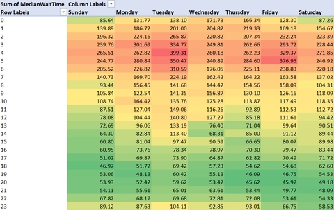
    DayOfWeekNum, Hour; -- Sort by numeric day of the week and hour

Plugging this into an Excel PivotTable (with a bit of conditional formatting magic), we can see the following:

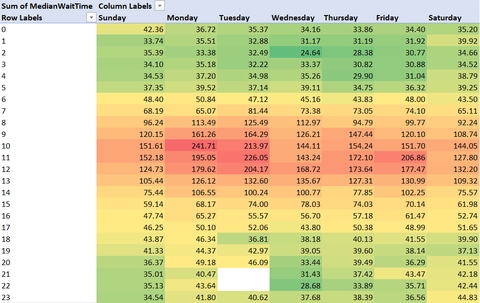
Heatmap for daily and hourly wait times for BTB Sentry Defense during Anvil.

Looks like if you are on the US West Coast, playing from 10AM UTC (3AM PT) is the worst - everyone is sleeping, and you might be waiting for more than two minutes to find a match.

What data is captured?

There are many factors that determine the wait times. The values provided by Halo Infinite services are an approximation, and the actual wait times can be shorter or longer than the declared value.

But you know what, this was a featured playlist. Would the data be different for, say, Ranked Arena? Let’s adjust the query above for the playlist with asset ID of EDFEF3AC-9CBE-4FA2-B949-8F29DEAFD483 and version ID of 6404AC75-0D91-46F8-929B-FE975A1ABDB4.

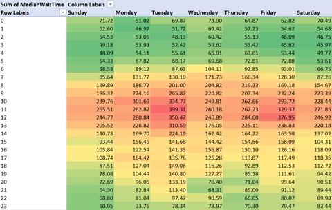
Heatmap for daily and hourly wait times for Ranked Arena during Anvil.

Looks like the best time to play Ranked Arena on the US West Coast is in the evening or late at night. Or so it would appear - a Reddit user observed a slight issue with the query above if we want to draw raw conclusions.

The conversion of timestamps using strftime will, by default, compute the data in UTC time. What that means is that the times rendered in the heatmap will be off by about 7 hours (offset for the PT timezone). To fix that, we need to use localtime to ensure that the timestamp is converted to the local machine time where the query is executed:

WITH HourlyWaitTimes AS (
    SELECT
        CASE strftime('%w', datetime(SnapshotTimestamp), 'localtime')
            WHEN '0' THEN 'Sunday'
            WHEN '1' THEN 'Monday'
            WHEN '2' THEN 'Tuesday'
            WHEN '3' THEN 'Wednesday'
            WHEN '4' THEN 'Thursday'
            WHEN '5' THEN 'Friday'
            WHEN '6' THEN 'Saturday'
        END AS DayOfWeek,
        strftime('%w', datetime(SnapshotTimestamp), 'localtime') AS DayOfWeekNum,
        strftime('%H', datetime(SnapshotTimestamp), 'localtime') AS Hour,
        WaitTime
    FROM
        WaitTimeSnapshots
    WHERE
        AssetId = 'EDFEF3AC-9CBE-4FA2-B949-8F29DEAFD483' AND
        VersionId = '6404AC75-0D91-46F8-929B-FE975A1ABDB4'
),
RankedWaitTimes AS (
    SELECT
        DayOfWeek,
        DayOfWeekNum,
        Hour,
        WaitTime,
        ROW_NUMBER() OVER (PARTITION BY DayOfWeek, Hour ORDER BY WaitTime) AS RowNum,
        COUNT(*) OVER (PARTITION BY DayOfWeek, Hour) AS TotalCount
    FROM
        HourlyWaitTimes
)
SELECT
    DayOfWeek,
    Hour,
    CASE
        WHEN TotalCount % 2 = 1 THEN MAX(WaitTime) -- Odd number of rows, middle one
        ELSE AVG(WaitTime) -- Even number of rows, average of the two middle values
    END AS MedianWaitTime
FROM
    RankedWaitTimes
WHERE
    RowNum IN ( (TotalCount + 1) / 2, (TotalCount + 2) / 2 )
GROUP BY
    DayOfWeek, Hour
ORDER BY
    DayOfWeekNum, Hour; -- Sort by numeric day of the week and hour

This would yield the following numbers:

Heatmap for daily and hourly median wait times for Ranked Arena during Anvil, snapped to local time.

Looks like the worst times to play are early mornings, and the best are in the afternoon, with more night opportunities on Friday and Saturday.

You can do similar analysis (and more) for any of the playlists that were active during an operation - all within the same database.

Feedback

The data for Fleetcom is being aggregated as we speak. Once the operation ends, you will see a new dataset drop in the OpenSpartan/waittimes-datasets repository.

If you have any questions, comments, or feedback - feel free to leave a note on this blog post, or open an issue on GitHub.